Mastering the Doughnut Chart in Excel: A Complete Information
Associated Articles: Mastering the Doughnut Chart in Excel: A Complete Information
Introduction
With nice pleasure, we’ll discover the intriguing matter associated to Mastering the Doughnut Chart in Excel: A Complete Information. Let’s weave attention-grabbing data and provide contemporary views to the readers.
Desk of Content material
Mastering the Doughnut Chart in Excel: A Complete Information
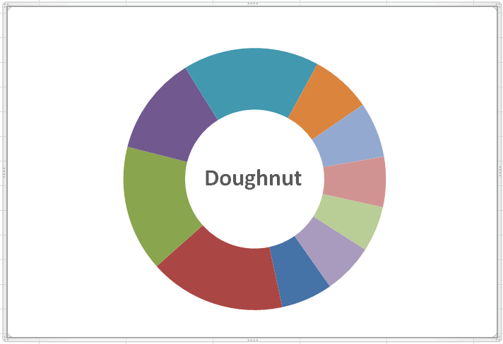
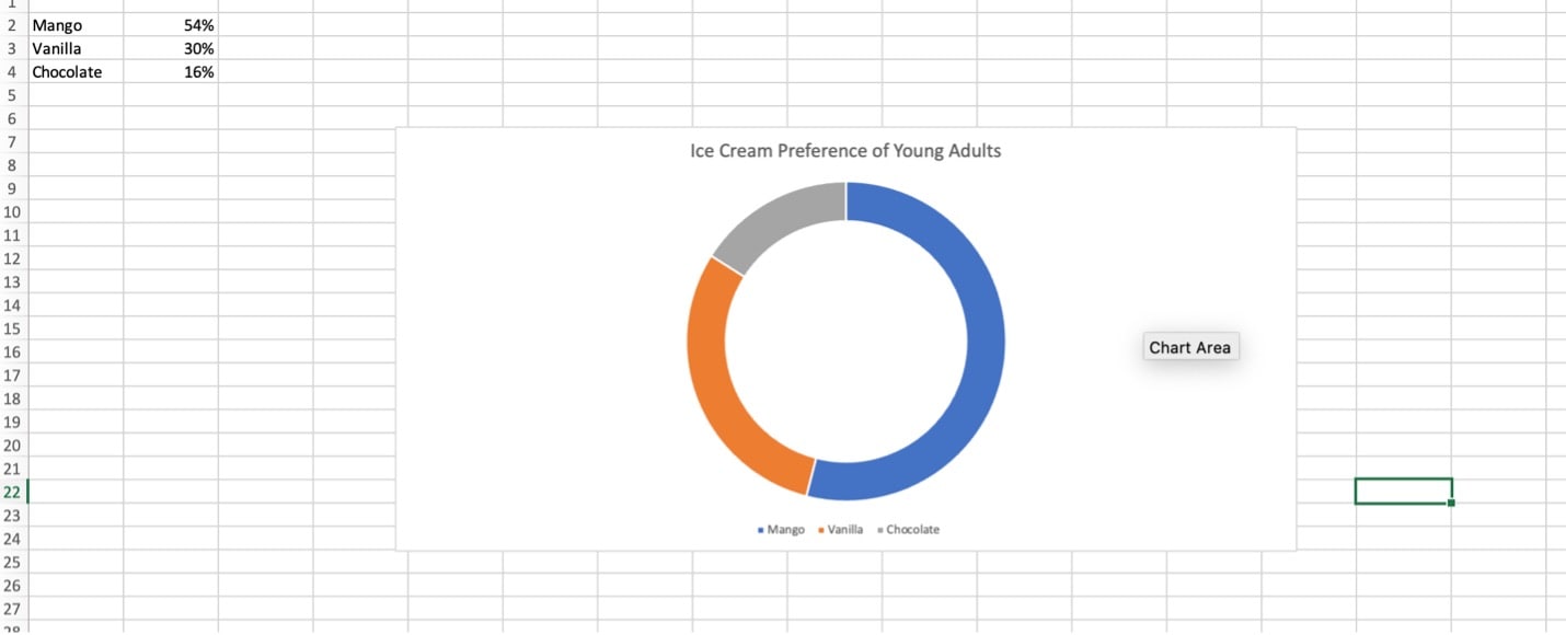
Doughnut charts, a visually interesting variation of pie charts, are wonderful for displaying proportional information throughout a number of classes. Not like pie charts, doughnut charts provide the added benefit of accommodating a central area, good for including labels, titles, or perhaps a smaller secondary chart. This information gives a complete walkthrough on creating and customizing gorgeous doughnut charts in Microsoft Excel, protecting all the things from primary creation to superior formatting strategies.
Half 1: Making ready Your Knowledge
Earlier than diving into chart creation, meticulously organizing your information is paramount. A well-structured dataset ensures a transparent and simply comprehensible chart. For a doughnut chart, your information needs to be introduced in two columns (or rows, relying in your choice):
- Class: This column lists the completely different classes for which you are displaying proportions. As an example, should you’re charting gross sales by product, this column would checklist every product. Guarantee every class is exclusive.
- Worth: This column comprises the numerical information representing the dimensions or proportion of every class. This might be gross sales figures, percentages, counts, or some other quantifiable information.
Instance Dataset:
| Product | Gross sales (USD) |
|---|---|
| Product A | 15000 |
| Product B | 10000 |
| Product C | 7500 |
| Product D | 5000 |
| Product E | 2500 |
Half 2: Creating the Fundamental Doughnut Chart
-
Choose Your Knowledge: Spotlight each the "Class" and "Worth" columns in your Excel sheet, making certain all information is included.
-
Insert Chart: Navigate to the "Insert" tab on the Excel ribbon. Within the "Charts" group, find the "Pie or Doughnut" charts. Choose the "Doughnut" chart possibility. Excel will mechanically generate a primary doughnut chart primarily based in your chosen information.
-
Preliminary Chart Look: Excel’s default formatting is a place to begin. The chart will show every class as a phase of the doughnut, with the dimensions of every phase proportional to its worth. The legend will mechanically label every phase with its corresponding class.
Half 3: Enhancing Your Doughnut Chart: Formatting and Customization
Whereas the essential chart is useful, vital enhancements may be made to reinforce its visible enchantment and readability. This part particulars superior formatting strategies:
1. Knowledge Labels: Clearly labeling every phase is essential. Proper-click on a phase throughout the chart and choose "Add Knowledge Labels." Experiment with completely different label positions (inside, exterior, greatest match) and formatting choices (share, worth, class title, or mixtures thereof). Think about including chief strains to attach labels to their respective segments for higher readability, particularly with many classes.
**2. Chart


Closure
Thus, we hope this text has offered invaluable insights into Mastering the Doughnut Chart in Excel: A Complete Information. We thanks for taking the time to learn this text. See you in our subsequent article!